5. A Posteriori Identifiability Analysis
Biological models are often highly complex which results in some parameters being unindentifiable. Identifiability analysis can be performed a posteriori to check if the parameters are well constrained. This example is similar to Example 3 but we now run the sampler multiple times to see if the parameters converge to the same region.
First, we import the required modules.
[1]:
import matplotlib.pyplot as plt
import numpy             as np
import pandas            as pd


import BMSS.models.model_handler as mh
import BMSS.models.setup_cf      as sc
import BMSS.icanalysis           as ac
import BMSS.curvefitting         as cf
import BMSS.traceanalysis        as ta
Connected to MBase_models, UBase_models
Connected to MBase_settings, UBase_settings
Next we import the models. In this case, we have three models that we want to fit:
A model for protein expression that lumps translation and trscription together i.e. no mRNA
[system_type]
system_type = LogicGate, Not, Single

[states]
states = p1, p2

[parameters]
parameters = kp1, synp1, synp2, rep, degp

[inputs]
inputs = u1

[equations]
equations =
    dp1 = synp1 *u1                    -degp*p1
    dp2 = synp2 *(kp1+rep*p1)/(kp1+p1) -degp*p2


[LogicGate, Not, Single]

init =
    p1 = [0],
    p2 = [0]

guess =
    kp1   = [5e-5],
    synp1 = [1e-5],
    synp2 = [1e-5],
    rep   = [0.8],
    degp  = [0.012],
    u1    = [0]

priors =
    degp = [0.012, 0.04]

parameter_bounds =
    kp1    = [1e-7, 1e-4],
    synp1  = [1e-7, 1e-4],
    synp2  = [1e-7, 1e-4],
    rep    = [0, 1],
    degp   = [0.001, 0.05],
    u1     = [0, 1]

input_conditions =
    u1 = 3

fixed_parameters =
    [degp, u1]

measured_states =
    [p1, p2]

decomposition =
    [[p1, p2]]

units =
    kp1   = M,
    synp1 = M/min,
    synp2 = M/min,
    rep   = NONE,
    degp  = 1/min,
    u1    = NONE
A model that includes mRNA transcription.
[system_type]
system_type = LogicGate, Not, Double

[states]
states = m1, m2, p1, p2

[parameters]
parameters = synm1, synm2, degm, kp1, rep, synp1, synp2, degp

[inputs]
inputs = u1

[equations]
equations =
    dm1 = synm1*u1                    -degm*m1
    dm2 = synm2*(kp1+rep*p1)/(kp1+p1) -degm*m2
    dp1 = synp1 *m1                   -degp*p1
    dp2 = synp2 *m2                   -degp*p2

[LogicGate, Not, Double]

init =
    m1 = [0],
    m2 = [0],
    p1 = [0],
    p2 = [0]

guess =
    synm1  = [1e-5],
    synm2  = [1e-5],
    degm   = [0.15],
    kp1    = [5e-5],
    rep    = [0.8],
    synp1  = [1e-2],
    synp2  = [1e-2],
    degp   = [0.012],
    u1     = [0]

priors =
    degm = [0.15, 0.05],
    degp = [0.012, 0.04]

parameter_bounds =
    synm1  = [1e-7, 1e-4],
    synm2  = [1e-7, 1e-4],
    degm   = [0.01, 0.3],
    kp1    = [1e-7, 1e-4],
    rep    = [0, 1],
    synp1  = [1e-3, 1e-1],
    synp2  = [1e-3, 1e-1],
    degp   = [0.001, 0.05],
    u1     = [0, 1]

input_conditions =
    u1 = 3

fixed_parameters =
    [degm, degp, u1]

measured_states =
    [p1, p2]

decomposition =
    [[m1, p1], [m2, p2]]

units =
    synm1  = M/min,
    synm2  = M/min,
    degm   = 1/min,
    kp1    = M,
    rep    = NONE,
    synp1  = 1/min,
    synp2  = 1/min,
    degp   = 1/min,
    u1     = NONE
A model that includes mRNA transcription and protein maturation.
[system_type]
system_type = LogicGate, Not, Double, MaturationSecond

[states]
states = m1, m2, p1, p2n, p2

[parameters]
parameters = synm1, synm2, degm, kp1, rep, synp1, synp2, matp2, degp

[inputs]
inputs = u1

[equations]
equations =
    dm1  = synm1*u1                    -degm *m1
    dm2  = synm2*(kp1+rep*p1)/(kp1+p1) -degm *m2
    dp1  = synp1 *m1                   -degp *p1
    dp2n = synp2 *m2                   -matp2*p2n
    dp2  = matp2*p2n                   -degp *p2

[LogicGate, Not, Double, MaturationSecond]

init =
    m1  = [0],
    m2  = [0],
    p1  = [0],
    p2n = [0],
    p2  = [0]

guess =
    synm1 = [1e-5],
    synm2 = [1e-5],
    degm  = [0.15],
    kp1   = [5e-5],
    rep   = [0.8],
    synp1 = [1e-2],
    synp2 = [1e-2],
    matp2 = [0.03],
    degp  = [0.012],
    u1    = [0]

priors =
    degm = [0.15, 0.05],
    degp = [0.012, 0.04]

parameter_bounds =
    synm1  = [1e-7, 1e-4],
    synm2  = [1e-7, 1e-4],
    degm   = [0.01, 0.3],
    kp1    = [1e-7, 1e-4],
    rep    = [0, 1],
    synp1  = [1e-3, 1e-1],
    synp2  = [1e-3, 1e-1],
    matp2  = [1e-3, 1e-1],
    degp   = [0.001, 0.05],
    u1     = [0, 1]

input_conditions =
    u1 = 3

fixed_parameters =
    [degm, matp2, degp, u1]

measured_states =
    [p1, p2]

decomposition =
    [[m1, p1], [m2, p2n, p2]]

units =
    synm1 = M/min,
    synm2 = M/min,
    degm  = 1/min,
    kp1   = M,
    rep   = NONE,
    synp1 = 1/min,
    synp2 = 1/min,
    matp2 = 1/min,
    degp  = 1/min,
    u1    = NONE
[2]:
#Set up core models and sampler arguments
#Details in Tutorial 5 Parts 1 and 2
model_files = ['LogicGate_Not_Single.ini',
               'LogicGate_Not_Double.ini',
               'LogicGate_Not_Double_MaturationSecond.ini',
               ]

user_core_models = [mh.from_config(filename) for filename in model_files]
user_core_models = {core_model['system_type']: core_model for core_model in user_core_models}

sampler_args, config_data = sc.get_sampler_args(model_files, user_core_models=user_core_models)
To characterize a NOT gate, we need to simulate the on and off states (i.e. two scenarios). Since we the parameter u0 will change depending on the scenario, we define a modify_params function that changes u0 based on the scenario. In addition, the initial values of the proteins in the models that include mRNA depend on the intial mRNA concentrations (assuming steady-state). We therefore also define a modify_init function that adjusts the initial values of the proteins based on the calculated steady-state values from the parameters.
[3]:
def modify_params(init_values, params, model_num, scenario_num, segment):
    #Always use a copy and not the original
    new_params = params.copy()

    #Change value of inducer based on scenario_num
    if scenario_num == 1:
        new_params[-1] = 0
    else:
        new_params[-1] = 1

    return new_params

def modify_init(init_values, params, model_num, scenario_num, segment):
    #Always use a copy and not the original
    new_init = init_values.copy()

    if model_num == 1:
        pass

    elif model_num == 2:
       synm1, synm2, degm, kp1, rep, synp1, synp2, degp, u1 = params

       new_init[1] = synm2/degm

    else:
        synm1, synm2, degm, kp1, rep, synp1, synp2, matp2, degp, u1 = params
        m1, m2, p1, p2n, p2 = init_values

        new_init[1] = synm2/degm
        new_init[3] = synp2*m2/matp2

    return new_init
Next we read the data. BMSS2 does not have a standardized file format for experimental data format. You have to write your own function to generate the appropriate data structures from your files.
[4]:
#This is just an example. Write your own based on your data file formats!
from   read_data                 import read_data

data_files = {'Fluor/OD' : 'data/not_gate.csv',
              }
data_mu, data_sd, init, state_sd, tspan = read_data(data_files, n_models=len(config_data))
Firstly, you will need data_mu, a dictionary containing the experimental means nested according to model_num->state->scenario_num.
Note: Scenario numbers in BMSS are always positive integers.
[5]:
data_mu[1]['Fluor/OD'][1]
[5]:
array([0.00016846, 0.00016709, 0.00016505, 0.00016492, 0.00016622,
       0.00016536, 0.0001663 , 0.00016791, 0.00016922, 0.00017165,
       0.0001749 , 0.0001772 , 0.00018073, 0.00018408, 0.00018661,
       0.00019042, 0.00019291, 0.00019494, 0.00019687, 0.0001982 ,
       0.00019873, 0.00020043, 0.00020122, 0.00020297, 0.00020254,
       0.00020265, 0.00020256, 0.0002019 , 0.00020067, 0.00019887,
       0.00019843, 0.0001972 , 0.00019612, 0.00019529, 0.00019439,
       0.00019349, 0.00019359, 0.00019448, 0.00019419, 0.00019417,
       0.00019455, 0.00019394, 0.00019388, 0.00019477, 0.00019417,
       0.00019461, 0.00019436, 0.00019537, 0.0001953 , 0.00019483,
       0.00019447, 0.00019562, 0.00019583, 0.00019644, 0.00019749,
       0.00019768, 0.00019793, 0.00019992, 0.00020136, 0.00020248,
       0.00020349, 0.00020434, 0.00020496, 0.00020666, 0.00020748,
       0.00020831, 0.00020953, 0.00021106, 0.00021324, 0.00021478,
       0.00021544, 0.00021685, 0.0002173 ])
For curve-fitting, 0 and -1 are are reserved for the time points and optional metadata respectively.
[6]:
data_mu[1]['Fluor/OD'][0]
[6]:
array([  0,  10,  20,  30,  40,  50,  60,  70,  80,  90, 100, 110, 120,
       130, 140, 150, 160, 170, 180, 190, 200, 210, 220, 230, 240, 250,
       260, 270, 280, 290, 300, 310, 320, 330, 340, 350, 360, 370, 380,
       390, 400, 410, 420, 430, 440, 450, 460, 470, 480, 490, 500, 510,
       520, 530, 540, 550, 560, 570, 580, 590, 600, 610, 620, 630, 640,
       650, 660, 670, 680, 690, 700, 710, 720], dtype=int64)
[7]:
data_mu[1]['Fluor/OD'][-1]
[7]:
['Time(min)', 'Input0', 'Input1']
Next we have data_sd, which represents the standard deviation for the data points. This is required for plotting. Like data_mu, it is a nested dictionary too.
[8]:
data_sd[1]['Fluor/OD'][1]
[8]:
array([2.42656e-06, 9.37248e-07, 9.19792e-07, 2.76109e-06, 3.24705e-06,
       4.98056e-07, 1.28286e-06, 3.47485e-07, 1.39350e-06, 1.39600e-06,
       2.72240e-06, 1.70335e-06, 2.02147e-06, 2.49997e-06, 1.24595e-06,
       2.04816e-06, 1.06684e-06, 2.64642e-06, 1.85434e-06, 2.66398e-06,
       3.28476e-06, 3.31294e-06, 3.41525e-06, 3.99973e-06, 4.00629e-06,
       4.72510e-06, 4.48240e-06, 4.34397e-06, 3.83979e-06, 3.96017e-06,
       3.44663e-06, 3.69322e-06, 3.21070e-06, 3.94781e-06, 4.10837e-06,
       3.72995e-06, 3.81588e-06, 3.91394e-06, 3.95898e-06, 3.69636e-06,
       2.62381e-06, 2.85074e-06, 3.24365e-06, 2.78016e-06, 3.04043e-06,
       3.42828e-06, 3.40368e-06, 3.31324e-06, 3.52927e-06, 3.18079e-06,
       3.70341e-06, 3.77066e-06, 3.90530e-06, 3.98203e-06, 4.34979e-06,
       2.97448e-06, 3.39774e-06, 3.83076e-06, 4.06592e-06, 3.39255e-06,
       3.40962e-06, 2.72869e-06, 3.80955e-06, 2.94705e-06, 3.21857e-06,
       3.25478e-06, 3.17322e-06, 2.91145e-06, 3.01634e-06, 3.46067e-06,
       3.16760e-06, 2.67769e-06, 3.34911e-06])
[9]:
data_sd[1]['Fluor/OD'][0]
[9]:
array([  0,  10,  20,  30,  40,  50,  60,  70,  80,  90, 100, 110, 120,
       130, 140, 150, 160, 170, 180, 190, 200, 210, 220, 230, 240, 250,
       260, 270, 280, 290, 300, 310, 320, 330, 340, 350, 360, 370, 380,
       390, 400, 410, 420, 430, 440, 450, 460, 470, 480, 490, 500, 510,
       520, 530, 540, 550, 560, 570, 580, 590, 600, 610, 620, 630, 640,
       650, 660, 670, 680, 690, 700, 710, 720], dtype=int64)
For curve-fitting, a standard deviation is required to normalize the SSE for each state.
[10]:
state_sd
[10]:
{'Fluor/OD': 2.1642987945205473e-06}
In the event the tspan and initial values in the settings file are not the same as the experimental data, you will have to reassign them in your script.
Now we update the sampler arguments with the information from the experimental data.
[11]:
#Update sampler_args with the information from the data
sampler_args['models'][1]['states'] = ['p1', 'Fluor/OD']
sampler_args['models'][2]['states'] = ['m1', 'm2', 'p1', 'Fluor/OD']
sampler_args['models'][3]['states'] = ['m1', 'm2', 'p1', 'p2n', 'Fluor/OD']
sampler_args['data']                = data_mu

for model_num in sampler_args['models']:
    sampler_args['models'][model_num]['tspan'] = [tspan]
    sampler_args['models'][model_num]['sd']    = state_sd

    model_init = {scenario: [init[model_num][scenario].get(state, 0) for state in sampler_args['models'][model_num]['states']] for scenario in init[model_num]}
    sampler_args['models'][model_num]['init']                      = model_init
    sampler_args['models'][model_num]['int_args']['modify_params'] = modify_params
    sampler_args['models'][model_num]['int_args']['modify_init']   = modify_init
Time to run the sampler! In this case, we’ll add a seeding function to make the sample start from a diffirent initial guess each time.
[12]:
def seed(guess, fixed_parameters, parameter_bounds):
    def vary(key):#Generate new value for parameter
        value = guess[key]
        delta = (np.random.rand() - 0.5)

        new_value            = value*16**delta#4 fold variation
        min_value, max_value = parameter_bounds.get(key, [None, None])

        if min_value is not None: #Make sure new value does not exceed bounds
            return max(min_value, min(max_value, new_value))
        else:
            return new_value

    def helper(return_original=False):
        if return_original:#Have a way to retrieve original guess
            return guess
        else:
            return {key: guess[key] if key in fixed_parameters else vary(key) for key in guess }
    return helper

seeder = seed(sampler_args['guess'], sampler_args['fixed_parameters'], sampler_args['bounds'])
[13]:
#Run sampler
traces    = {}#To collect the trace

for i in range(5):
    sampler_args['guess'] = seeder()
    result    = cf.simulated_annealing(**sampler_args)
    steps     = result['all']
    traces[i] = steps
100%|██████████████████████████████████████████████████████████████████████████████| 3000/3000 [00:32<00:00, 91.58it/s]
100%|██████████████████████████████████████████████████████████████████████████████| 3000/3000 [00:36<00:00, 83.13it/s]
100%|█████████████████████████████████████████████████████████████████████████████| 3000/3000 [00:27<00:00, 107.35it/s]
100%|█████████████████████████████████████████████████████████████████████████████| 3000/3000 [00:22<00:00, 135.94it/s]
100%|█████████████████████████████████████████████████████████████████████████████| 3000/3000 [00:22<00:00, 136.33it/s]
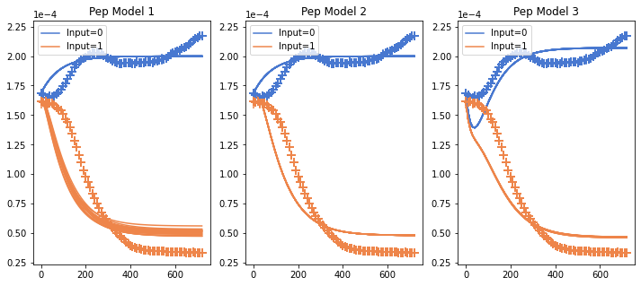
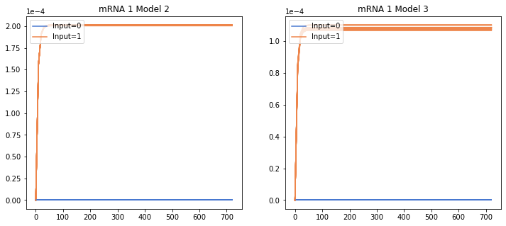
After fitting, we plot the results to check the fit.
[14]:
#Plot results
plt.rcParams['figure.figsize'] = [12, 5]
plt.rcParams['figure.subplot.hspace'] = 0.99

plot_index  = {1: ['Fluor/OD'],
               2: ['Fluor/OD', 'm1', 'm2'],
               3: ['Fluor/OD', 'm1', 'm2',]
               }
titles      = {1: {'Fluor/OD': 'Pep Model 1'},
               2: {'Fluor/OD': 'Pep Model 2', 'm1': 'mRNA 1 Model 2', 'm2': 'mRNA 2 Model 2'},
               3: {'Fluor/OD': 'Pep Model 3', 'm1': 'mRNA 1 Model 3', 'm2': 'mRNA 2 Model 3'}
               }
labels      = {1: {1: 'Input=0', 2: 'Input=1'},
               2: {1: 'Input=0', 2: 'Input=1'},
               3: {1: 'Input=0', 2: 'Input=1'}
               }
legend_args = {'loc': 'upper left'}

accepted  = result['a']
figs, AX  = cf.plot(posterior   = accepted.iloc[-40::2],
                    models      = sampler_args['models'],
                    data        = data_mu,
                    data_sd     = data_sd,
                    plot_index  = plot_index,
                    labels      = labels,
                    titles      = titles,
                    legend_args = legend_args,
                    figs        = None,
                    AX          = None
                    )
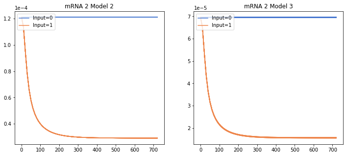
A Posteriori Identifiability Analysis
We can check the trace plots to determine if the parameters have been identified. If a parameter that has been successfully identified, its trace will show that the sampler converges to the same region for each run. For a quantitative approach, we can use R-hat to determine the ratio of variance within chains and between chains.
[15]:
plt.rcParams['figure.figsize'] = [10, 10]

trace_params = [p for p in accepted.columns if p not in sampler_args['fixed_parameters']]
n_figs       = round(len(trace_params)/8 + 0.5)
trace_figs   = [plt.figure() for i in range(n_figs)]
trace_AX_    = [trace_figs[i].add_subplot(4, 2, ii+1) for i in range(len(trace_figs)) for ii in range(8)]
trace_AX     = dict(zip(trace_params, trace_AX_))

trace_figs, trace_AX = ta.plot_steps(traces,
                                     skip        = sampler_args['fixed_parameters'],
                                     legend_args = legend_args,
                                     figs        = trace_figs,
                                     AX          = trace_AX
                                     )
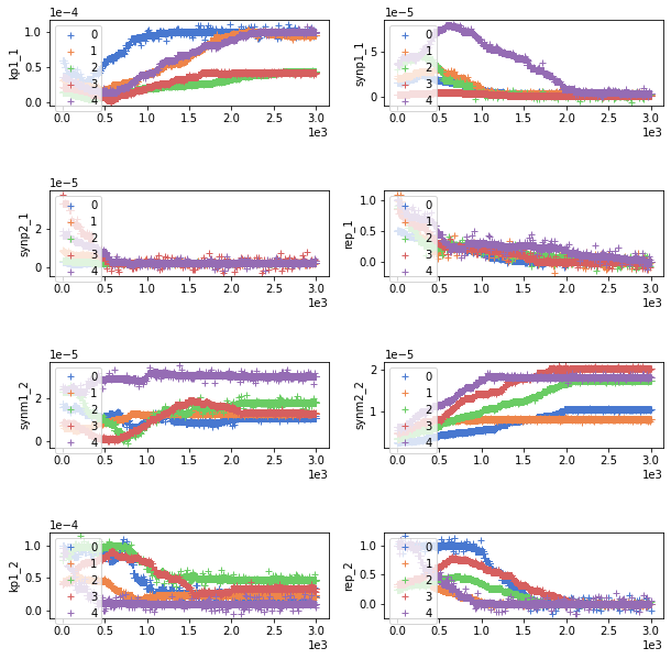
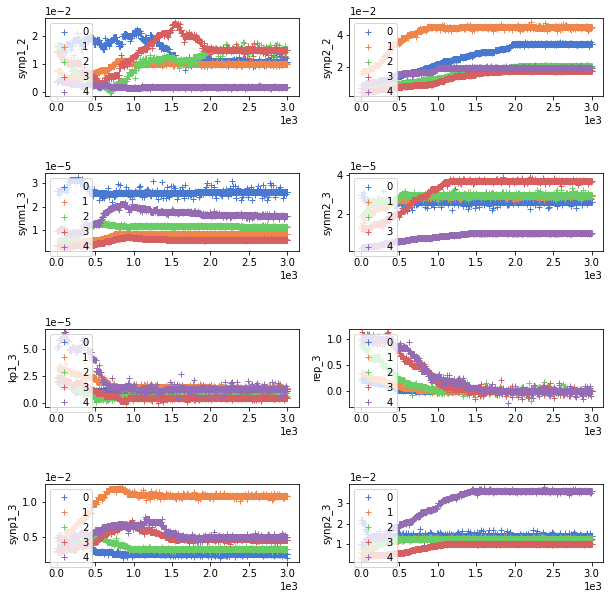
[16]:
rhat = ta.calculate_rhat(traces, skip=sampler_args['fixed_parameters'])
[17]:
rhat
[17]:
kp1_1      2.120985
synp1_1    2.393335
synp2_1    1.341627
rep_1      1.921702
synm1_2    2.027821
synm2_2    2.270518
kp1_2      2.042286
rep_2      1.993550
synp1_2    2.068563
synp2_2    2.276792
synm1_3    2.607740
synm2_3    2.252711
kp1_3      1.643786
rep_3      1.821316
synp1_3    2.760944
synp2_3    2.817088
dtype: float64
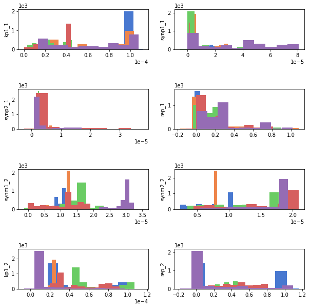
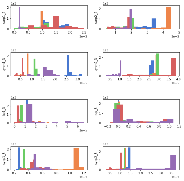
We can also check the distribution of the parameters for each run by calling the plot_hist or plot_kde functions.
[18]:
hist_figs   = [plt.figure() for i in range(n_figs)]
hist_AX_    = [hist_figs[i].add_subplot(4, 2, ii+1) for i in range(len(hist_figs)) for ii in range(8)]
hist_AX     = dict(zip(trace_params, hist_AX_))

hist_figs, hist_AX = ta.plot_hist(traces, skip=sampler_args['fixed_parameters'], figs=hist_figs, AX=hist_AX)