2. Simulate New Model
In this example, we show you to perform a simple simulation in BMSS2.
Basic Simulation
The steps for analyzing a model not in the database are as follows:
Read the settngs file with BMSS.models.setup_sim.from_config
Read the core model file with BMSS.models.model_handler.from_config
Get the arguments required for analysis with BMSS.models.get_models_and_params
[1]:
import matplotlib.pyplot as plt
import os
import pandas  as pd
from   numba   import jit
from   pathlib import Path


import BMSS.models.model_handler as mh
import BMSS.models.setup_sim     as sm
import BMSS.simulation           as sim
Connected to MBase_models, UBase_models
Connected to MBase_settings, UBase_settings
After importing the modules, we call the functions read the config files. These are files in .ini format where you specify the topology of the model and the settings for simulation and other types of analysis.
First we have the file that specifies the topology of the model
[system_type]
system_type = TestModel, Dummy

[states]
states = m, p

[parameters]
parameters = k_ind, synm, degm, synp, degp

[inputs]
inputs = ind

[equations]
equations =
    dm = synm*ind/(ind + k_ind) - degm*m
    dp = synp*m - degp*p
Next we have the file which specifies the settings for simulation.
[TestModel, Dummy]

init =
    m = [0, 1e-4],
    p = [0, 1e-4]

parameter_values =
    k_ind = [1e-2, 5e-2],
    synm  = [1e-5]*2,
    degm  = [0.015]*2,
    synp  = [1e-2]*2,
    degp  = [0.012]*2,
    ind   = [8e-2]*2

tspan =
    [0, 600, 61]

#Optional
solver_args =
    rtol   = 1.49012e-08,
    atol   = 1.49012e-08
Note: BMSS2 uses numpy’s odeint for integration. To tweak settings such as step size or tolerance, add an optional solver_args section in the settings file to specify the optional parameters of odeint. These include, rtol, atol, tcrit, h0, hmax, hmin, mxstep.
[2]:
#Read model
core_model       = mh.from_config('testmodel.ini')
user_core_models = {core_model['system_type']: core_model}

#Read settings
filename    = 'settings_sim_1.ini'
config_data = sm.from_config(filename)

#Get arguments for simulation
models, params, config_data = sm.get_models_and_params(filename, user_core_models=user_core_models)
At this point, we can call perform the simulation by calling the integrate_models function.
The results of the integration are stored in ym as a nested dictionary in the form of ym[model_num][scenario_num][row] where row is a row index in params. Meanwhile, ym[model_num][0] contains the time array for the model. Thus, suppose we only have one model. ym will then have one key. If that model has 2 scenarios, ym[1] will have 2 keys not including 0. Finally, if there are two rows of parameters, ym[1][1] and ym[1][2] will have two keys each.
[3]:
ym, _ = sim.integrate_models(models, params)

print('Keys in ym:', ym.keys())
print('Keys in ym[1]', ym[1].keys())
print('Keys in ym[1][1]', ym[1][1].keys())
Simulating models
Simulation complete
Keys in ym: dict_keys([1])
Keys in ym[1] dict_keys([1, 2, 0])
Keys in ym[1][1] dict_keys([0])
The following arguments follow a similar format to models where the first key corresponds to the model being integrated. The definition of the values indexed by those keys are as follows:
plot_index : A list of state variables to plot as well as extra functions for plotting.
titles : A list of title names corresponding the states in plot_index. This argument is optional.
labels : A dict of scenario: name pairs that will be used in the legend. This argument is optional.
[4]:
plot_index  = {1: ['m', 'p'],
               }
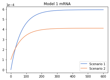
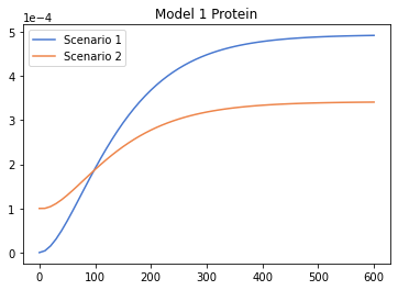
titles      = {1: {'m': 'Model 1 mRNA', 'p': 'Model 1 Protein'},
               }
labels      = {1: {1: 'Scenario 1', 2: 'Scenario 2'}
               }

figs, AX = sim.plot_model(plot_index, ym, titles=titles, labels=labels)
Plotting extra variables
Sometimes, we might want to examine quantities that are not time series of the state variables. In this case, we can come up with our own functions to evaluate extra variables. This extra function takes of the form of func(y, t, params). The arrays in ym and their corresponding rows in params are fed into this function. The return values are:
The y axis values
The x axis values
The marker used for plotting (Refer to matplotlib)
[5]:
@jit(nopython=True)
def synthesis_p(y, t, params):
    '''
    filler
    x: Time
    y: synthesis_rate
    filler
    '''
    m = y[:,0]

    synp = params[3]

    synthesis_rate = synp*m

    return synthesis_rate, t, '-'

ym, em = sim.integrate_models(models, params, synthesis_p)
Simulating models
Simulation complete
Note that em is a nested dictinary in the form em[function][model_num][scenario_num][row]
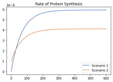
To plot the synthesis rate, modify the plot settings accordingly.
[6]:
plot_index  = {1: ['p', synthesis_p],
               }
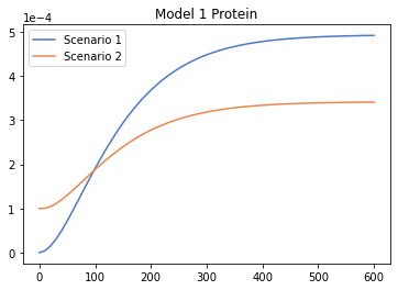
titles      = {1: {'p': 'Model 1 Protein', synthesis_p: 'Rate of Protein Synthesis'},
               }
labels      = {1: {1: 'Scenario 1', 2: 'Scenario 2'}
               }

figs, AX = sim.plot_model(plot_index, ym, e=em, titles=titles, labels=labels)
Finally, we can export the data for our external analysis in csv format.
[7]:
#Prefix at the front of the filenames
prefix = ''

#A new folder will be created using this directory. The files will be stored here.
directory = Path(os.getcwd()) / 'simulation_results'

sim.export_simulation_results(ym, em, prefix=prefix, directory=directory)
[7]:
['y_1_1_0.csv',
 'y_1_2_1.csv',
 'synthesis_p_1_1_0.csv',
 'synthesis_p_1_2_1.csv']
[8]:
pd.read_csv('simulation_results/y_1_1_0.csv')
[8]:
| Unnamed: 0 | Time | m | p | |
|---|---|---|---|---|
| 0 | 0 | 0.0 | 0.000000 | 0.000000 |
| 1 | 1 | 10.0 | 0.000083 | 0.000004 |
| 2 | 2 | 20.0 | 0.000154 | 0.000015 |
| 3 | 3 | 30.0 | 0.000215 | 0.000031 |
| 4 | 4 | 40.0 | 0.000267 | 0.000050 |
| ... | ... | ... | ... | ... |
| 56 | 56 | 560.0 | 0.000592 | 0.000491 |
| 57 | 57 | 570.0 | 0.000592 | 0.000492 |
| 58 | 58 | 580.0 | 0.000592 | 0.000492 |
| 59 | 59 | 590.0 | 0.000593 | 0.000492 |
| 60 | 60 | 600.0 | 0.000593 | 0.000492 |
61 rows × 4 columns
Piecewise Integration
BMSS2 also allows piecewise integration where the tspan field is broken into multiple lists. For example, a list of [0, 100, 11] could be broken in to [0, 50, 6], [50, 100, 6]. The user can define a custom function in their Python script to be passed into BMSS under the “modify_init” or “modify_param” argument which will modify the states or parameters between segments.
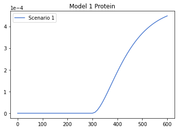
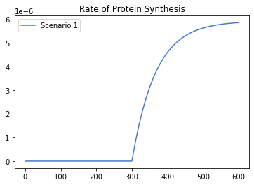
Supposed the inducer is added at a certain time point. We can simulate this by:
Breaking the tspan argument into segments
Adding a modify_param
[9]:
def change_inducer_by_scenario_and_segment(init_values, params, model_num, scenario_num, segment):
        '''
        Modifies the the current array of params based on model_num, scenario, segment and init_values.
        '''

        new_params   = params.copy()
        if model_num == 1 and segment == 1 and scenario_num == 1:
            new_params[-1] = 8e-2

        return new_params
Now we import the settings
[TestModel, Dummy]

init =
    m   = [0],
    p   = [0]

parameter_values =
    k_ind = [1e-2],
    synm  = [1e-5],
    degm  = [0.015],
    synp  = [1e-2],
    degp  = [0.012],
    ind   = [0]

units =
    k_ind = % Arabinose,
    synm  = M/min,
    degm  = 1/min,
    synp  = M/min,
    degp  = 1/min,
    ind   = % Arabinose

tspan =
    [0, 300, 31], [300, 600, 31]
[10]:
filename = 'settings_sim_2.ini'
models, params, config_data = sm.get_models_and_params(filename)

#Print tspan
print('Tspan for two-segment experiment')
print(models[1]['tspan'])

#Modify models accordingly
models[1]['int_args']['modify_params'] = change_inducer_by_scenario_and_segment
Tspan for two-segment experiment
[array([  0.,  10.,  20.,  30.,  40.,  50.,  60.,  70.,  80.,  90., 100.,
       110., 120., 130., 140., 150., 160., 170., 180., 190., 200., 210.,
       220., 230., 240., 250., 260., 270., 280., 290., 300.]), array([300., 310., 320., 330., 340., 350., 360., 370., 380., 390., 400.,
       410., 420., 430., 440., 450., 460., 470., 480., 490., 500., 510.,
       520., 530., 540., 550., 560., 570., 580., 590., 600.])]
[11]:
#Integrate
ym, em = sim.integrate_models(models, params, synthesis_p)

figs, AX = sim.plot_model(plot_index, ym, e=em, titles=titles, labels=labels)
Simulating models
Simulation complete
Note that the initial values can also be modified in a similar manner. Write your own function and place it under models[model_num][‘int_args’][‘modify_init’] instead.